Machine Learning Lecture 2¶

Abstract: These exercises will familiarize with more advanced machine learning concepts including hyperparameter tuning and cross-validation. You will also see how to visualize the model that is learned by a machine learning classifier.

Strategies for Preventing Overfitting: Regularization

Last time we discussed machine learning we examined the tradeoff of the number of training examples and the performance of the model on predicting new instances. We did this by producing graphs of model performance as a function of the amount of training data used:

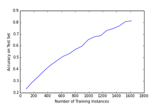
This graph shows the performance of a logistic regression model at predicting which of digit is represented by an 8 pixel by 8 pixel grayscale image of a hand written digit.

While it is nice that the model’s performance increases as we add more data, it would be nice if there was a way to have it all: better performance with less data. Fortunately, many machine learning algorithms have strategies that attempt to achieve this goal. Consider the objective function of the standard logistic regression model that we talked about a couple of lectures ago:

We can augment this objective with a term that serves to penalize large weights (i.e. large values of the entries of w). This modification serves to reduce the flexibility of fitting the training data, thereby improving the performance on predicting future data. The modified objective function is:

Where C is a positive constant that balance how much we care about fitting the training data compared to penalizing large weights. To understand this a bit better, let’s consider the limiting behavior. How would this new version of logistic regression behave as C goes to 0? How about as C goes to infinity?

We can rerun our experiment on learning to recognize handwritten digits with this modified version of logistic regression. For starters, let’s just use the default value of C=1. The learning curve now looks like this:

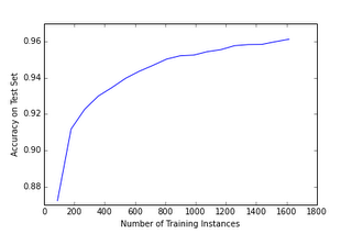
Woah! This is a lot better… However, we might ask ourselves whether we can do even better if we tuned the value of C a little bit.

Tuning Hyper Parameters

It turns out that properly tuning the values of constants such as C (the penalty for large weights in the logistic regression model) is perhaps the most important skill for successfully applying machine learning to a problem. Let’s see how this learning curve will look with different values of C:

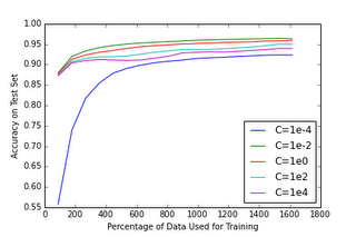
If we zoom in a bit on the more interesting part of the graph:

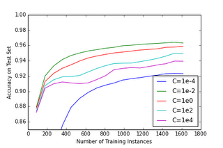
It looks like we can do a bit better than the default value of C=1 by choosing C=0.01. How well do would we expect our model to do on predicting images of handwritten digits if we were to collect a brand new database?

Luckily, Scikit-learn provides some built-in mechanisms for doing parameter tuning in a sensible manner. One such method is to use a cross validation to choose the optimal setting of a particular parameter.

Cross validation can be performed in scikit-learn using the following code:

from sklearn.cross_validation import train_test_split
from sklearn.grid_search import GridSearchCV
from sklearn.datasets import *
from sklearn.linear_model import LogisticRegression

data = load_digits()

tuned_parameters = [{'C': [10**-4, 10**-2, 10**0, 10**2, 10**4]}]
X_train, X_test, y_train, y_test = train_test_split(data.data, data.target, train_size=.9)

model = GridSearchCV(LogisticRegression(), tuned_parameters, cv=5)
model.fit(X_train, y_train)

print model.best_estimator_
print model.score(X_test, y_test)

LogisticRegression(C=1, class_weight=None, dual=False, fit_intercept=True,
          intercept_scaling=1, penalty=l2, random_state=None, tol=0.0001)
0.955555555556

Visualizing the Learned Model

In some cases it may be informative to examine the pattern of weights learned by a machine learning model. This visualization can either be useful for understanding your data in a new way, or as a method of creating new features in order to improve model performance.

To visualize how the logistic regression model discriminates between the various classes of digits, we use the following code:

%matplotlib inline
from sklearn.datasets import *
import matplotlib.pyplot as plt
import numpy
from sklearn.linear_model import LogisticRegression

data = load_digits()
model = LogisticRegression()
model.fit(data.data, data.target)

fig = plt.figure()

for i in range(10):
    subplot = fig.add_subplot(5,2,i+1)
    subplot.matshow( numpy.reshape(model.raw_coef_[i][1:], (8,8)), cmap='gray')

plt.show()

Non-linear Models

Now that we have learned the basics of the process of applying a particular machine learning algorithm (logistic regression), we can start to explore more advanced machine learning algorithms. There are probably hundreds of machine learning algorithms for every step of the machine learning pipeline. Scikit learn has some of the built-in (check out the documentation here). Next, I will briefly show how we can apply a new machine learning algorithm to the task of classifying digits.

A very powerful machine learning algorithm is the support vector machine (or SVM). Part of the reason that this algorithm is so powerful is that it is capable of learning non-linear decision boundaries.

In order to apply the support vector machine to the digit classification problem, we need to intelligently tune the parameters of the algorithm (or else we will get suboptimal performance). In contrast the logistic regression model, the support vector machine has more hyper parameters to tune. Here is a snippet of code that tunes the parameters of a support vector machine:

from sklearn.cross_validation import train_test_split
from sklearn.grid_search import GridSearchCV
from sklearn.datasets import *
from sklearn.linear_model import LogisticRegression
from sklearn.svm import SVC

data = load_digits()

tuned_parameters = [{'kernel': ['rbf'],'gamma': [1e-3, 1e-4], 'C': [1, 10, 100, 1000]},
                    {'kernel': ['linear'], 'C': [1, 10, 100, 1000]}]


X_train, X_test, y_train, y_test = train_test_split(data.data, data.target, train_size=0.9)
model = GridSearchCV(SVC(C=1), tuned_parameters, cv=5)

model.fit(X_train, y_train)

print model.best_estimator_
print model.score(X_test, y_test)

SVC(C=1, cache_size=200, class_weight=None, coef0=0.0, degree=3, gamma=0.001,
  kernel=rbf, max_iter=-1, probability=False, random_state=None,
  shrinking=True, tol=0.001, verbose=False)
0.994444444444

Experiment with other built-in scikit-learn classifiers. For instance, can you use a similar methodology as above but instead apply k-nearest neighbors or random forests? Try this out in the cell below. Which method appears to do the best?